CERN Accelerating science

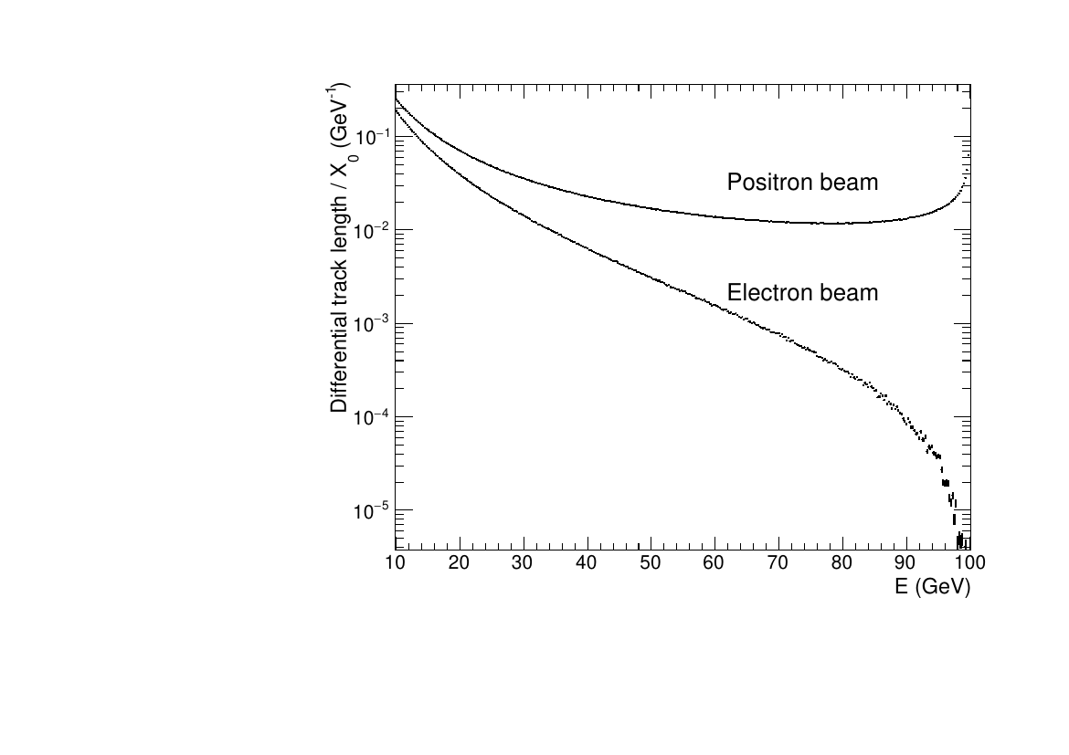Differential track length $\frac{dT_+}{dE}$ of positrons in a thick target, for a 100 GeV electron and positron beam. In the electron case, only secondary $e^+$ contribute to $\frac{dT_+}{dE}$, resulting in a monotone, decreasing track length, dominated by low energy positrons; on the other hand, an $e^+$ beam results in a significantly larger $\frac{dT_+}{dE}$, peaked at $E_{beam}$, due to the primary particle contribution.

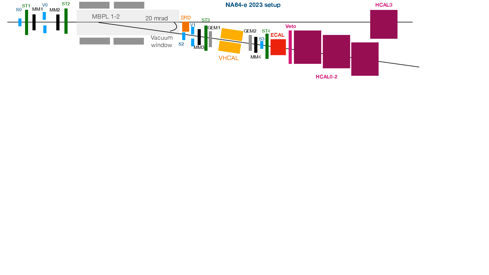Overview of the NA64 experimental setup for the 2023 data-taking.

Overview of the NA64 experimental setup for the 2023 data-taking.

Illustration of a typical pile-up event measured during the NA64-2023 $e^+$ run. The left, middle, right plot show, respectively, the measured waveform for the central SRD cell, the central ECAL cell, and the central HCAL0 cell. In each plot, the vertical red line corresponds to the measured peak time $t_0$, while the three red rectangles are centered at the expected time $t_E$ and correspond, respectively, to the $\pm1$ $\sigma_{t_E}$, $\pm2$ $\sigma_{t_E}$, $\pm3$ $\sigma_{t_E}$ intervals. The ECAL signal clearly shows a double-peak structure, with a first small in-time pulse, followed by a larger one. The HCAL signal (right) shows a single in-time pulse. Finally, the SRD signal (left) also shows a single pulse, that is, however, at a much larger time than the expected one. This event can be explained as the superposition of a proton impinging first on the detector, followed immediately after by a positron. The proton passed through the ECAL with a small energy deposition therein and then released all its energy in the HCAL, with no associated activity in the SRD. The positron, instead, resulted in a visible energy deposition in the SRD, and a large signal in the ECAL.

Illustration of a typical pile-up event measured during the NA64-2023 $e^+$ run. The left, middle, right plot show, respectively, the measured waveform for the central SRD cell, the central ECAL cell, and the central HCAL0 cell. In each plot, the vertical red line corresponds to the measured peak time $t_0$, while the three red rectangles are centered at the expected time $t_E$ and correspond, respectively, to the $\pm1$ $\sigma_{t_E}$, $\pm2$ $\sigma_{t_E}$, $\pm3$ $\sigma_{t_E}$ intervals. The ECAL signal clearly shows a double-peak structure, with a first small in-time pulse, followed by a larger one. The HCAL signal (right) shows a single in-time pulse. Finally, the SRD signal (left) also shows a single pulse, that is, however, at a much larger time than the expected one. This event can be explained as the superposition of a proton impinging first on the detector, followed immediately after by a positron. The proton passed through the ECAL with a small energy deposit therein and then released all its energy in the HCAL, with no associated activity in the SRD. The positron, instead, resulted in a visible energy deposit in the SRD, and a large signal in the ECAL.

Illustration of a typical pile-up event measured during the NA64-2023 $e^+$ run. The left, middle, right plot show, respectively, the measured waveform for the central SRD cell, the central ECAL cell, and the central HCAL0 cell. In each plot, the vertical red line corresponds to the measured peak time $t_0$, while the three red rectangles are centered at the expected time $t_E$ and correspond, respectively, to the $\pm1$ $\sigma_{t_E}$, $\pm2$ $\sigma_{t_E}$, $\pm3$ $\sigma_{t_E}$ intervals. The ECAL signal clearly shows a double-peak structure, with a first small in-time pulse, followed by a larger one. The HCAL signal (right) shows a single in-time pulse. Finally, the SRD signal (left) also shows a single pulse, that is, however, at a much larger time than the expected one. This event can be explained as the superposition of a proton impinging first on the detector, followed immediately after by a positron. The proton passed through the ECAL with a small energy deposition therein and then released all its energy in the HCAL, with no associated activity in the SRD. The positron, instead, resulted in a visible energy deposition in the SRD, and a large signal in the ECAL.

Illustration of a typical pile-up event measured during the NA64-2023 $e^+$ run. The left, middle, right plot show, respectively, the measured waveform for the central SRD cell, the central ECAL cell, and the central HCAL0 cell. In each plot, the vertical red line corresponds to the measured peak time $t_0$, while the three red rectangles are centered at the expected time $t_E$ and correspond, respectively, to the $\pm1$ $\sigma_{t_E}$, $\pm2$ $\sigma_{t_E}$, $\pm3$ $\sigma_{t_E}$ intervals. The ECAL signal clearly shows a double-peak structure, with a first small in-time pulse, followed by a larger one. The HCAL signal (right) shows a single in-time pulse. Finally, the SRD signal (left) also shows a single pulse, that is, however, at a much larger time than the expected one. This event can be explained as the superposition of a proton impinging first on the detector, followed immediately after by a positron. The proton passed through the ECAL with a small energy deposit therein and then released all its energy in the HCAL, with no associated activity in the SRD. The positron, instead, resulted in a visible energy deposit in the SRD, and a large signal in the ECAL.

Illustration of a typical pile-up event measured during the NA64-2023 $e^+$ run. The left, middle, right plot show, respectively, the measured waveform for the central SRD cell, the central ECAL cell, and the central HCAL0 cell. In each plot, the vertical red line corresponds to the measured peak time $t_0$, while the three red rectangles are centered at the expected time $t_E$ and correspond, respectively, to the $\pm1$ $\sigma_{t_E}$, $\pm2$ $\sigma_{t_E}$, $\pm3$ $\sigma_{t_E}$ intervals. The ECAL signal clearly shows a double-peak structure, with a first small in-time pulse, followed by a larger one. The HCAL signal (right) shows a single in-time pulse. Finally, the SRD signal (left) also shows a single pulse, that is, however, at a much larger time than the expected one. This event can be explained as the superposition of a proton impinging first on the detector, followed immediately after by a positron. The proton passed through the ECAL with a small energy deposition therein and then released all its energy in the HCAL, with no associated activity in the SRD. The positron, instead, resulted in a visible energy deposition in the SRD, and a large signal in the ECAL.

Illustration of a typical pile-up event measured during the NA64-2023 $e^+$ run. The left, middle, right plot show, respectively, the measured waveform for the central SRD cell, the central ECAL cell, and the central HCAL0 cell. In each plot, the vertical red line corresponds to the measured peak time $t_0$, while the three red rectangles are centered at the expected time $t_E$ and correspond, respectively, to the $\pm1$ $\sigma_{t_E}$, $\pm2$ $\sigma_{t_E}$, $\pm3$ $\sigma_{t_E}$ intervals. The ECAL signal clearly shows a double-peak structure, with a first small in-time pulse, followed by a larger one. The HCAL signal (right) shows a single in-time pulse. Finally, the SRD signal (left) also shows a single pulse, that is, however, at a much larger time than the expected one. This event can be explained as the superposition of a proton impinging first on the detector, followed immediately after by a positron. The proton passed through the ECAL with a small energy deposit therein and then released all its energy in the HCAL, with no associated activity in the SRD. The positron, instead, resulted in a visible energy deposit in the SRD, and a large signal in the ECAL.

Left panel: average energy deposit in the ECAL for events recorded by the prescaled ``calibration-trigger'' condition, for each production run. For each data point, the error bar corresponds to a $\pm 1\sigma$ for the corresponding distribution. Right panel: the reconstructed momentum distribution from tracking detectors for all the calibration events. The distribution was fitted with a Gaussian function.

Left panel: average energy deposit in the ECAL for events recorded by the prescaled ``calibration-trigger'' condition, for each production run. For each data point, the error bar corresponds to a $\pm 1\sigma$ for the corresponding distribution. Right panel: the reconstructed momentum distribution from tracking detectors for all the calibration events. The distribution was fitted with a Gaussian function.

Left: total energy deposited in all SRD modules by positron (blue) / hadron (red) events. The vertical black line corresponds to the 2.5 MeV cut employed in the analysis. Right: SRD detector efficiency for impinging 70 GeV/c $e^+$ (black) / false-positive probability for hadrons (red) as a function of the energy threshold -- for most of the data points, the size of the error bar is smaller than the marker.

Left: total energy deposited in all SRD modules by positron (blue) / hadron (red) events. The vertical black line corresponds to the 2.5 MeV cut employed in the analysis. Right: SRD detector efficiency for impinging 70 GeV/c $e^+$ (black) / false-positive probability for hadrons (red) as a function of the energy threshold -- for most of the data points, the size of the error bar is smaller than the marker.

2D distribution of the $\chi^2$ versus the measured energy in the ECAL, for the collected di-muon events.

Efficiency of the HCAL cut, defined as $E_{HCAL} < E_{HCAL}^{threshold}$, where $E_{HCAL}$ is the total energy deposited in the three modules, as a function of the threshold applied to the total energy deposited in the first three modules. The error bars on the $y$ axis are covered by the marker size.

Left (right) panel: ECAL efficiency $\eta_{ECAL}(m_\Apr)$ for $\Apr$ signal events from $e^+e^-$ annihilation as a function of the pre-shower (ECAL) energy threshold, for different dark photon masses. Both the plots refer to the case $\alpha_D=0.1$.

Left (right) panel: ECAL efficiency $\eta_{ECAL}(m_\Apr)$ for $\Apr$ signal events from $e^+e^-$ annihilation as a function of the pre-shower (ECAL) energy threshold, for different dark photon masses. Both the plots refer to the case $\alpha_D=0.1$.

Top-left panel: the ECAL energy spectrum for 70 GeV/c positrons selected by the upstream cuts in a production run (blue) and in a calibration run (red), both scaled to unity in the 20-40 GeV range. Top-right panel: the ratio of the two distributions, together with an unbinned maximum likelihood fit performed with a sigmoidal function to extract the value of the ECAL missing energy trigger threshold $E_{thr}$. Lower panel: the ECAL energy distribution of all events selected after applying all the analysis cuts, together with the result of an extended maximum-likelihood fit performed with an exponential function multiplied by a sigmoidal to evaluate the expected background yield due to upstream interactions. We underline that in the 42-46 GeV range no events have been observed. See text for further details.

Left panel: the ECAL energy spectrum for 70 GeV/c positrons selected by the upstream cuts in a production run (blue) and in a calibration run (red), both scaled to unity in the 20-40 GeV range. Right panel: the ratio of the two distributions, together with an unbinned maximum likelihood fit performed with a sigmoidal function to extract the value of the ECAL missing energy trigger threshold $E_{thr}$. Lower panel: the ECAL energy distribution of all events selected after applying all the analysis cuts, together with the result of a fit performed with an exponential function to evaluate the expected background yield due to upstream interactions. We underline that in the 42-46 GeV range no events have been observed.

Top-left panel: the ECAL energy spectrum for 70 GeV/c positrons selected by the upstream cuts in a production run (blue) and in a calibration run (red), both scaled to unity in the 20-40 GeV range. Top-right panel: the ratio of the two distributions, together with an unbinned maximum likelihood fit performed with a sigmoidal function to extract the value of the ECAL missing energy trigger threshold $E_{thr}$. Lower panel: the ECAL energy distribution of all events selected after applying all the analysis cuts, together with the result of an extended maximum-likelihood fit performed with an exponential function multiplied by a sigmoidal to evaluate the expected background yield due to upstream interactions. We underline that in the 42-46 GeV range no events have been observed. See text for further details.

Left panel: the ECAL energy spectrum for 70 GeV/c positrons selected by the upstream cuts in a production run (blue) and in a calibration run (red), both scaled to unity in the 20-40 GeV range. Right panel: the ratio of the two distributions, together with an unbinned maximum likelihood fit performed with a sigmoidal function to extract the value of the ECAL missing energy trigger threshold $E_{thr}$. Lower panel: the ECAL energy distribution of all events selected after applying all the analysis cuts, together with the result of a fit performed with an exponential function to evaluate the expected background yield due to upstream interactions. We underline that in the 42-46 GeV range no events have been observed.

Top-left panel: the ECAL energy spectrum for 70 GeV/c positrons selected by the upstream cuts in a production run (blue) and in a calibration run (red), both scaled to unity in the 20-40 GeV range. Top-right panel: the ratio of the two distributions, together with an unbinned maximum likelihood fit performed with a sigmoidal function to extract the value of the ECAL missing energy trigger threshold $E_{thr}$. Lower panel: the ECAL energy distribution of all events selected after applying all the analysis cuts, together with the result of an extended maximum-likelihood fit performed with an exponential function multiplied by a sigmoidal to evaluate the expected background yield due to upstream interactions. We underline that in the 42-46 GeV range no events have been observed. See text for further details.

Left: HCAL vs ECAL energy distribution for $K^+$ in-flight decay events. Right: ECAL energy distribution for $\mu^+$ in-flight decay events, normalized to single impinging muon.

Di-muon events HCAL energy distribution distributions for different ECAL energy intervals, together with the result of the fit with an exponential curve used to extrapolate the yield in the low-energy region.

Di-muon events HCAL energy distribution distributions for different ECAL energy intervals, together with the result of the fit with an exponential curve used to extrapolate the yield in the low-energy region.

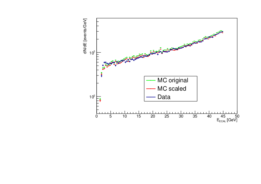Comparison of the dimuons yield for data (blue) and Monte Carlo. The green histogram shows the MC spectrum scaled according to Eq.~\ref{eq:MC_Scaling_Dimuons}. The red histogram represents the MC spectrum scaled for an additional factor 0.93 to ensure a proper comparison between the data and the simulation.

Comparison of the di-muons yield for data (blue) and MC. The green histogram shows the MC spectrum scaled according to Eq.~\ref{eq:MC_Scaling_Dimuons}. The red histogram represents the MC spectrum scaled for an additional factor 0.93. For data, the energy range $E_{ECAL} \gtrsim 50$~GeV shows the effect of the ECAL trigger threshold.

Events distribution in the $E_{HCAL}$ vs $E_{ECAL}$ space after the all selection cuts. The red rectangle highlights the signal region (the Y-axis extent is enlarged by a factor of 4 for better visibility).

Exclusion limits at 90\% confidence level derived from the 70 GeV/c positron-beam missing energy measurement presented in this work. Top (bottom): exclusion limits - brown and orange curves- in the $[m_\Apr,\varepsilon]$ ($[m_\chi,\alpha_D]$) plane, for $\alpha_D$ = 0.1 (left) and $\alpha_D$ = 0.5 (right). The other curves and shaded areas report already-existing limits in the same parameters space from NA64 in electron-beam mode~\cite{Andreev:2023uwc} (blue and violet), COHERENT~\cite{COHERENT:2021pvd} (grey), and BaBar~\cite{BaBar:2016sci} (light blue). In the bottom plots, the black lines show the favored parameter combinations for the observed dark matter relic density for different variations of the model.

Exclusion limits at 90\% confidence level derived from the 70 GeV/c positron-beam missing energy measurement presented in this work. Top (bottom): exclusion limits - brown and orange curves- in the $[m_\Apr,\varepsilon]$ ($[m_\chi,\alpha_D]$) plane, for $\alpha_D$ = 0.1 (left) and $\alpha_D$ = 0.5 (right). The other curves and shaded areas report already-existing limits in the same parameters space from NA64 in electron-beam mode~\cite{Andreev:2023uwc} (blue and violet), COHERENT~\cite{COHERENT:2021pvd} (grey), and BaBar~\cite{BaBar:2016sci} (light blue). In the bottom plots, the black lines show the favored parameter combinations for the observed dark matter relic density for different variations of the model.

Exclusion limits at 90\% confidence level derived from the 70 GeV/c positron-beam missing energy measurement presented in this work. Top (bottom): exclusion limits - brown and orange curves- in the $[m_\Apr,\varepsilon]$ ($[m_\chi,\alpha_D]$) plane, for $\alpha_D$ = 0.1 (left) and $\alpha_D$ = 0.5 (right). The other curves and shaded areas report already-existing limits in the same parameters space from NA64 in electron-beam mode~\cite{Andreev:2023uwc} (blue and violet), COHERENT~\cite{COHERENT:2021pvd} (grey), and BaBar~\cite{BaBar:2016sci} (light blue). In the bottom plots, the black lines show the favored parameter combinations for the observed dark matter relic density for different variations of the model.

Exclusion limits at 90\% confidence level derived from the 70 GeV/c positron-beam missing energy measurement presented in this work. Top (bottom): exclusion limits - brown and orange curves- in the $[m_\Apr,\varepsilon]$ ($[m_\chi,\alpha_D]$) plane, for $\alpha_D$ = 0.1 (left) and $\alpha_D$ = 0.5 (right). The other curves and shaded areas report already-existing limits in the same parameters space from NA64 in electron-beam mode~\cite{Andreev:2023uwc} (blue and violet), COHERENT~\cite{COHERENT:2021pvd} (grey), and BaBar~\cite{BaBar:2016sci} (light blue). In the bottom plots, the black lines show the favored parameter combinations for the observed dark matter relic density for different variations of the model.

Projected sensitivity of the proposed positron measurements in the $(y,m_\chi)$ plane in the $(m_\chi,y)$ plane, for $\alpha_D=0.1$. The green and cyan curves are the results obtained from the detailed simulation of the 40 GeV and 60 GeV measurement, and the red curve corresponds to their combination.

Red (blue) markers: efficiency of the shower shape cut on resonant annihilation events simulated with $\alpha_D =0.1$ ($\alpha_D =0.5$), as a function of the $\Apr$ mass.

ECAL energy distribution for selected electro-/photo-nuclear upstream events: data (blue) vs MC prediction (red). The MC distribution is fitted with an exponential function $f(E_{ECAL})=\exp(-c_{const}+c_{slope}E_{ECAL})$ (in green) to assess the systematic uncertainty connected to the extrapolation of the upstream-interactions background yield(see Sec.~\ref{sec:upstreamInteractions} for details).